Introduction:

I'm an Aerodynamicist. That's been my main focus since I began college. I like to work on projects that directly involve aerodynamics or rely on my knowledge of the subject. Computational Fluid Dynamics (CFD) is one of the tools in my quiver. I've been doing CFD for about 13 years, deriving and writing my own models from scratch. Most of the systems I've created have been targeted to model specific flows. Each was developed from first principles, building from either the Navier-Stokes or Euler equations. I've made systems modeling internal and external flows operating in the subsonic, transonic and supersonic regimes. I've employed finite-difference and finite-volume approaches to descretize the physical domains. Most of my work has modeled unsteady flows, using time-accurate, time-marching schemes, but I have also written a few systems that advance the solution in time using implicit schemes. I've also thrown in one or two space-marching solutions for good measure. I've modeled frozen, equilibrium and nonequilibrium flows. For some of my work, I've developed systems with non-reflective boundaries. And for some problems, I've written systems using "upwind" schemes to calculate the gradients or fluxes.

Some Examples:

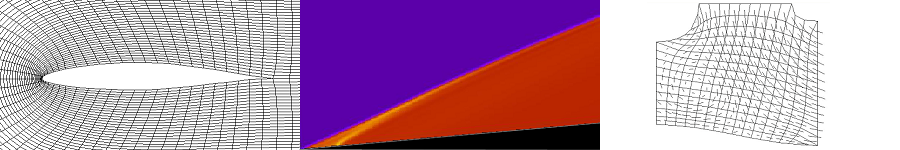
One of the systems I've written computes the 2-dimensional, viscous flow of air over a flat plate. The figure to the right shows a contour plot of Mach number from a run using the simulation to model the flow over a 5-degree wedge. The flow enters from the left at Mach 4. The strong shock wave that forms at the leading edge of the wedge is clearly visible. It turns the flow 5 degrees so that it is parallel with the upper surface of the wedge. There is an analytical solution to this problem--oblique shock wave theory--which assumes that the flow is inviscid. It predicts that the flow downstream of the shock should be at Mach 3.64. The results here are very close to that. Note how the viscous simulation captures the buildup of the boundary layer and also the shock structures that form around the leading edge of the wedge. (Click on any image on this page to see a larger version.) The center figure in the masthead of this page is the contour plot of pressure from the same simulation run. The pressure rises sharply as the air flows through the shock wave. The colors map just as they do in this figure, with yellow indicating high pressure and blue low. Note the shock structures around the leading edge of the wedge and the high pressures that form.

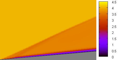
A very interesting application of the same simulation computes the supersonic, viscous flow of air over a flat plate. This sounds like a very simple flow scenario, but isn't. In fact, there is no "closed-form" or analytical solution to the problem. The only way to see what happens is to solve the problem numerically or experimentally. 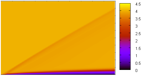The figure to the left is a contour plot of Mach number. Air enters from the left at Mach 4, and the flat plate forms the bottom edge of the figure. The buildup of the boundary layer is clearly visible above the flat plate. It causes a slight displacement of the main flow. A weak shock wave forms to turn the flow slightly away from the plate. What makes this problem interesting is that the boundary layer is the reason the shock wave forms. If the flow were inviscid, there would be no boundary layer and hence no shock wave at all. The whole flowfield would be at Mach 4, a pretty uninteresting solution. The CFD simulation is accurate enough to resolve a collection of very weak shock waves, commonly called "Mach waves", downstream of the first shock wave. Each of these forms to turn the flow slightly more, accounting for the ever-increasing growth of the boundary layer.

One of the greatest challenges that I've found in CFD is high temperature gas flows. These are found in hypersonic flows, reentry flows, combusting flows or other types of flows where the gas is raised to high temperatures. The theory behind these flows combines fluid mechanics with quantum mechanics. Now, that's a challenge! These flows almost always involve multiple species of gas in vibrational, chemical and electronic nonequilibrium. 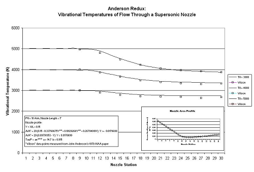I needed to incorporate high-temperature flow models into my engine simulation. Temperatures within the cylinder of a pistion engine reach 4,000° F (2,200 C). And exhaust flow temperatures can exceed 1,400° (760 C). Before incorporating these calculations into the engine simulation, I needed to see if I understood all of the high-temperature concepts and if I could apply them to a CFD solution. While at the Naval Ordinance Laboratory, John Anderson wrote a paper titled, "A Time-Dependent Analysis for Vibrational and Chemical Nonequilibrium Nozzle Flows". In it, he generates and presents data for a flow in vibrational nonequilibrium. I constructed my own CFD simulation incorporating vibrational nonequilibrium so that I could compare results. They are presented at the right. The figure represents the "vibrational temperature", a measure of the vibrational energy stored in diatomic nitrogen gas as it flows through a supersonic nozzle. The gas is stored at high temperature and pressure in a reservoir at the left side of the figure and then expands isentropically through the nozzle, to the exit at the right. As you can see from the plots, my system's predictions match the data from Anderson's paper very well.

No CFD simulation can work without a grid or mesh generator. I've written a number of them. The figure to the left shows a rectangular 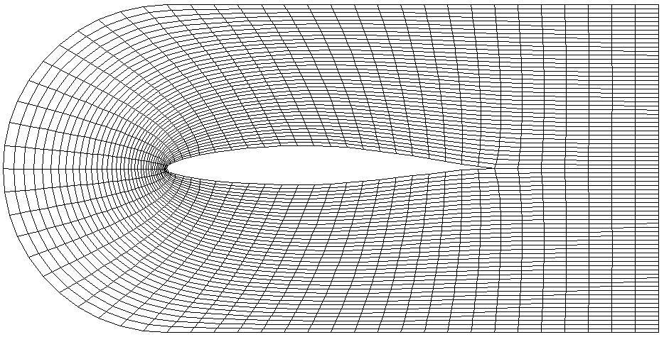mesh wrapped around an NACA 65-212 airfoil. The spatial location of the cell vertices at the airfoil surface and at the outer boundary is specified. The interior vertices are then distributed in space elliptically using the Laplace equation as a numerical artifice. The Laplace equation is solved across the physical domain using a finite difference approach. The system is mathematically elliptic in space and so I use a relaxation technique to drive the system to the steady state, as you see it here.

My engine simulation required a very special mesh generator. The engine simulation allows the user to connect intake and exhaust pipes together using a volume called a "collector". One requirement for the development of the simulation was that it not require the use of a CAD system when describing the layout of an intake or exhaust system. When a user 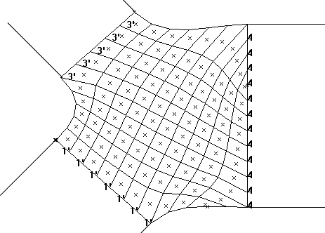wants to connect pipes together, he only needs to state which pipes, and which ends of those pipes, to connect together, and at what angles those pipes must meet. The simulation automatically generates a collector volume that will validly connect the pipes together. Then it automatically lays out a rectangular computational mesh inside of the volume. At the right, you see a collector that connects three pipes together. One pipe connects horizontally, from the right and two others connect at 45° and -45° angles from the left. The numbers indicate the pipe that each collector boundary cell connects to. The cells at the upper-left connect to pipe number 3. The primes on the numbers indicate that the cells connect to the "nth" end of the pipe; un-primed numbers indicate that the cells connect to the "0th" end. The shape of the collector wall between pipes is generated using a cubic spline. The location of cell vertices at the wall is laid-out uniformly. The spatial location of the interior vertices is then generated elliptically, using the Laplace equation as a numerical artifice. The "x" in each cell indicates the area centroid of the cell.

The figure at the left shows a collector in action, connecting three pipes together. An exhaust header pipe, connected to 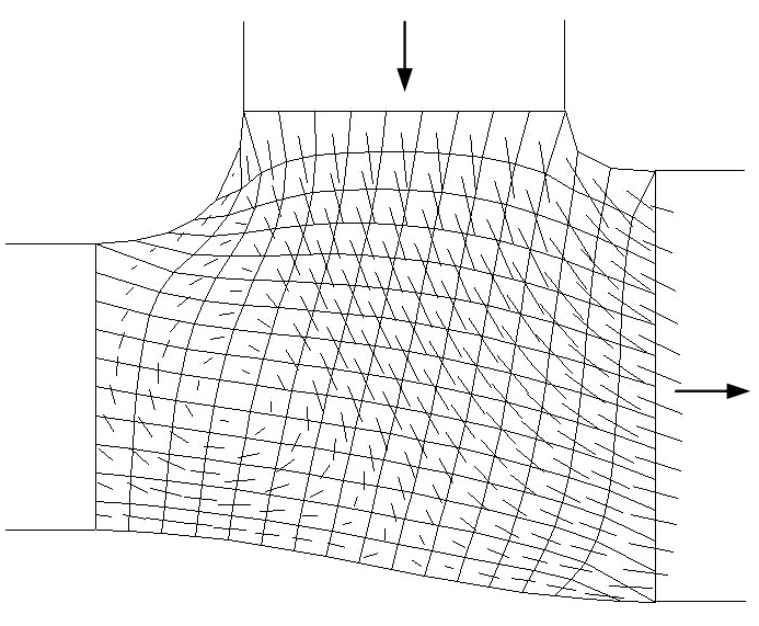a cylinder at its far end, joins vertically. Another header pipe connects horizontally from the left. A third exhaust pipe joins at the right, its far end open to the atmosphere. The exhaust valve at the far end of the left pipe is closed. The exhaust valve connecting the top pipe to its cylinder is open, and the piston is forcing the combustion charge out. The charge is flowing down that pipe and through the collector. The flow enters the collector and exits through the third pipe, toward the atmosphere. The collector's computational mesh and the velocity vectors at each cell are displayed. Because of the extreme computational constraints facing an engine simulation, the flow through the collector is modeled inviscidly. But note how the simulation is still able to resolve an area of recirculating flow near the connection to the left pipe. Also, note the stagnation point on the bottom wall. The flows within an engine are entirely unsteady. What you see here is just a snapshot in time.