Introduction:
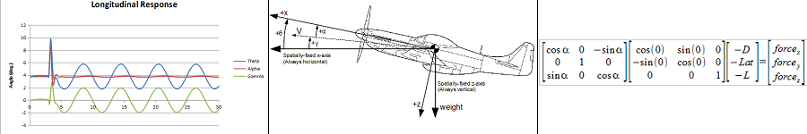
Over the years, I've written seven flight simulations. Looking back on them, I can see that each was written for a specific purpose. I love numerical modeling. Applying math and physics to a problem and working through a derivation to create a final model puts me in my natural habitat. Then I enjoy embodying that model in code and exercising it to get answers. For me, that's what Engineering is all about. The rigid body equations of motion, which all flight simulations are based on, are just such a system. When I first started writing flight simulations, I didn't fully understand them. In all of the texts I could find, the derivation of the equations was incomplete, with skipped steps and lots of confusing hand waving. In recent years, I've gone back, collecting as much as I could from disparate sources, and I now have the only complete derivation of the equations of motion that I've ever seen. It's liberating to finally understand them from front to back.
Naval Air Engineering Center:
The first flight simulation I wrote was in my first real engineering
job, in the Advanced Systems Group at the Naval Air Engineering
Center.
 We did a lot of Operations Research work in that branch, studying
complex systems, creating techniques for analyzing them, and then
improving or optimizing them. The paper at the right, written by
our Branch Head and his Deputy, is a good
example of that work. (Click on any image on this page to see
a larger version.) As one of our analysis tools in the branch,
I created a 3
degree-of-freedom flight simulation that predicted only the
longitudinal motion of an aircraft. The dynamic model included
catapult tow forces as well as constrained motion along a curved
surface. Using it, we could analyze the requirements that
different aircraft placed on the sizing and use of a catapult.
We could also see the effect that a curved, ski-jump shaped,
flight deck would have on the launch of any aircraft, and how
its use could affect the size of the flight deck and the length
of the catapult. Applying the program to foreign aircraft
carriers, we could predict the size of the largest aircraft
they could launch. I took the simulation with me to my next
assignment, in the Research and Development Department. There,
with some modifications, we used it to evaluate possible future
aircraft/ship combinations, to determine whether aircraft carrier
sizes could be reduced or mission effectiveness increased. I was
very pleased to find the program still in use by the department
a few years later. In its last incarnation--that I know of--I
used the same simulation as the basis for a Visual Landing
Aid design and analysis system. Combined with a pilot model and
a random number generator, we could use the system to analyze
aircraft carrier visual landing aids, generating touchdown point
distributions along the arresting portion of the flight deck.
That's a good amount of mileage from one simulation.
We did a lot of Operations Research work in that branch, studying
complex systems, creating techniques for analyzing them, and then
improving or optimizing them. The paper at the right, written by
our Branch Head and his Deputy, is a good
example of that work. (Click on any image on this page to see
a larger version.) As one of our analysis tools in the branch,
I created a 3
degree-of-freedom flight simulation that predicted only the
longitudinal motion of an aircraft. The dynamic model included
catapult tow forces as well as constrained motion along a curved
surface. Using it, we could analyze the requirements that
different aircraft placed on the sizing and use of a catapult.
We could also see the effect that a curved, ski-jump shaped,
flight deck would have on the launch of any aircraft, and how
its use could affect the size of the flight deck and the length
of the catapult. Applying the program to foreign aircraft
carriers, we could predict the size of the largest aircraft
they could launch. I took the simulation with me to my next
assignment, in the Research and Development Department. There,
with some modifications, we used it to evaluate possible future
aircraft/ship combinations, to determine whether aircraft carrier
sizes could be reduced or mission effectiveness increased. I was
very pleased to find the program still in use by the department
a few years later. In its last incarnation--that I know of--I
used the same simulation as the basis for a Visual Landing
Aid design and analysis system. Combined with a pilot model and
a random number generator, we could use the system to analyze
aircraft carrier visual landing aids, generating touchdown point
distributions along the arresting portion of the flight deck.
That's a good amount of mileage from one simulation.
Naval Air Development Center
Later, I transferred to the Navy's Flight Dynamics Branch at the
Naval Air Development Center.
There, they used flight simulations for their most basic
purpose--evaluating and improving aircraft flight dynamics,
 flying qualities and control harmony. They gave me the assignment
to create a new simulation for the group. The simulation
embodied a decoupled, 6 degree-of-freedom (3 DOF longitudinal,
3 DOF lateral/directional), linearized model.
flying qualities and control harmony. They gave me the assignment
to create a new simulation for the group. The simulation
embodied a decoupled, 6 degree-of-freedom (3 DOF longitudinal,
3 DOF lateral/directional), linearized model.
 They already had a coupled, 6 degree-of-freedom, non-linear
simulation in the group, and they wanted this new model for
comparison purposes. I wrote the report at the left on the
new simulation, comparing its predictions with those of the
non-linear model. The results were interesting. The linear
model would match the non-linear model during
a control deflection. But then, as one would expect, with
increasing simulated time, the linear response would slowly
diverge from the non-linear response. At the time that I wrote
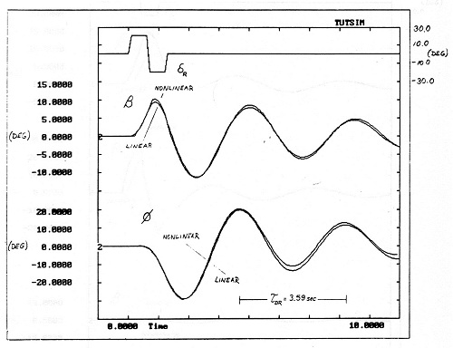
this simulation, the group was doing a lot of work with the
McDonnel-Douglas T-45 Goshawk. The figure to the right shows
one plot from the report: the T-45's response to a rudder
doublet, as predicted by both models. Note the small
differences in the responses and the
increasing difference between the curves as time marches on.
They already had a coupled, 6 degree-of-freedom, non-linear
simulation in the group, and they wanted this new model for
comparison purposes. I wrote the report at the left on the
new simulation, comparing its predictions with those of the
non-linear model. The results were interesting. The linear
model would match the non-linear model during
a control deflection. But then, as one would expect, with
increasing simulated time, the linear response would slowly
diverge from the non-linear response. At the time that I wrote
this simulation, the group was doing a lot of work with the
McDonnel-Douglas T-45 Goshawk. The figure to the right shows
one plot from the report: the T-45's response to a rudder
doublet, as predicted by both models. Note the small
differences in the responses and the
increasing difference between the curves as time marches on.

My next flight simulation was for a very focused purpose. I joined a group that was creating the world's first fully autonomous UAV control system. For our work, we needed a hardware-in-the-loop (HIL) simulation. That kind of simulation is used to make a system think that it is connected to a real device. In our case, we wanted our airborne control system to think that it was flying in a real airplane. With the HIL simulation, we could develop and test the airborne control system in the lab, on the workbench. I created a 6 degree-of-freedom, non-linear flight simulation of the UAV, and added to it realistic dynamic models of a gimbal and camera. Written carefully, I found that the simulation could run many times faster than real-time on our 20 MHz PC. We eventually increased the realism of the simulation even more by adding models, generating realistic errors and noise, of the sensors and actuators on the aircraft. Even with those added, it still ran faster than real-time. Here is a paper that I wrote on the simulation for a computer programming conference and a video of the simulation in action:
 The Sensor Driven Airborne Replanner Simulation
![]() The Sensor Driven Airborne Replanner simulation being used
for hardware-in-the-loop flight control system development.
The Sensor Driven Airborne Replanner simulation being used
for hardware-in-the-loop flight control system development.
Analytical Methods, Inc.
I recently wrote another hardware-in-the-loop simulation at Analytical Methods, Inc. That simulation was created for the laboratory development of their collapsible-wing, man-portable UAV. We had a full set of aerodynamic data for the aircraft, assembled from wind tunnel and CFD analyses. I wrote the simulation to sample that data at runtime, providing a fully nonlinear simulation that could reproduce the aircraft dynamics over the full range of airspeeds and attitudes, including departures from flight in the post-stall and spin regimes. Having never had a full aerodynamic data set to work with before, I was stunned by the realism of the simulation's responses.
Current Developments:
I'm currently creating a new flight simulation for my own use.
I've included all of the lessons I've learned from developing
past simulations and I can say that this is the best I've ever
developed. The simulation is intended for many different uses,
from open-loop, bare-airframe flight dynamics analyses to
hardware-in-the-loop
simulation.
It assumes a round, rather than flat, Earth model and
will correctly model a vehicle's dynamics from the surface up
through orbit, so it can be used on aircraft or rockets.
I've written the system so that new dynamic models,
of gimbals, servos, engines, sensors, etc., can be added with
very little effort. The program can communicate and be
controlled by any other program, because its interface is
the UDP stack. It will have a selection of "cabs" that can be
used to operate the simulation, from the keyboard and joystick,
from input files, from an A/D--D/A interface (for harware-in-the-loop
work) or any others that prove useful.
It will also have hooks to connect to
FlightGear and X-Plane, for use as visualization systems.
On my 2.13 GHz Pentium laptop, it currently runs
about 2,000 times real-time.
 So it's perfect for use in developing
intelligent systems, where full missions need to be flown or where
many
instances of the simulation (many aircraft, that is) need to be
simulated at one time.
The figure to the right is the output from a run controlled with
the open-loop cab. Here, I'm simulating a Cessna 150 trimmed at
an approach speed of 70 kts. A doublet input is applied to the
rudder and then the aircraft is allowed to respond. In the
"Body-Axis Velocities" plot, you can see the rudder input and the initial
response of the aircraft, as the lateral velocity (v) oscillates
and damps-out quickly. In the "Body-Axis Rotational Rates" and
"Lateral/Directional Displacements" plots, you can see the "dutch
roll" response of the aircraft, as motion around the vertical axis
is linked to the motion about the roll axis. Aircraft "heading" angle
is labeled "Psi", bank angle is labeled "Phi" and sideslip angle
is labeled "Beta". The dutch roll damps-out quickly, which is a
positive attribute for an aircraft, especially
a trainer. After the dutch roll damps out, the aircraft enters
into a spiral mode, as it rolls from the upright, accelerates and
begins descending. This mode would be dangerous if the airplane
were allowed to fly without any control input. But with a pilot
at the controls it's not an issue. The spiral mode diverges so
slowly that the pilot will correct for it without even knowing
that it's happening.
So it's perfect for use in developing
intelligent systems, where full missions need to be flown or where
many
instances of the simulation (many aircraft, that is) need to be
simulated at one time.
The figure to the right is the output from a run controlled with
the open-loop cab. Here, I'm simulating a Cessna 150 trimmed at
an approach speed of 70 kts. A doublet input is applied to the
rudder and then the aircraft is allowed to respond. In the
"Body-Axis Velocities" plot, you can see the rudder input and the initial
response of the aircraft, as the lateral velocity (v) oscillates
and damps-out quickly. In the "Body-Axis Rotational Rates" and
"Lateral/Directional Displacements" plots, you can see the "dutch
roll" response of the aircraft, as motion around the vertical axis
is linked to the motion about the roll axis. Aircraft "heading" angle
is labeled "Psi", bank angle is labeled "Phi" and sideslip angle
is labeled "Beta". The dutch roll damps-out quickly, which is a
positive attribute for an aircraft, especially
a trainer. After the dutch roll damps out, the aircraft enters
into a spiral mode, as it rolls from the upright, accelerates and
begins descending. This mode would be dangerous if the airplane
were allowed to fly without any control input. But with a pilot
at the controls it's not an issue. The spiral mode diverges so
slowly that the pilot will correct for it without even knowing
that it's happening.
I'll be using this simulation to create new UAV control systems. If you'd like to use it for your work, I intend to offer copies of the simulation for sale after it's complete. Stay tuned.